
Volume 13, Issue 1 (3-2025)
Jorjani Biomed J 2025, 13(1): 44-52 |
Back to browse issues page


Download citation:
BibTeX | RIS | EndNote | Medlars | ProCite | Reference Manager | RefWorks
Send citation to:


BibTeX | RIS | EndNote | Medlars | ProCite | Reference Manager | RefWorks
Send citation to:
Nosrati M, Yaghoubi M. Presenting a neural network-based framework for drug-target interaction prediction. Jorjani Biomed J 2025; 13 (1) :44-52
URL: http://goums.ac.ir/jorjanijournal/article-1-1078-en.html
URL: http://goums.ac.ir/jorjanijournal/article-1-1078-en.html


1- Department of Computer Engineering, Faculty of Engineering, Golestan University, Gorgan, Iran
2- Department of Computer Engineering, Faculty of Engineering, Golestan University, Gorgan, Iran ,mehdi.yaghoubi@gmail.com
2- Department of Computer Engineering, Faculty of Engineering, Golestan University, Gorgan, Iran ,
Keywords: Drug Delivery Systems, Convolutional Neural Networks, 3D structure, Graph Attention Network
Full-Text [PDF 944 kb]
(697 Downloads)
| Abstract (HTML) (5086 Views)
Lee et al. (14), in 2019, presented a deep learning model named DeepConv-DTI for predicting drug-target interactions by identifying and analyzing local residual patterns of proteins. This model uses convolutional neural networks on raw protein sequences to detect protein binding sites for drug-target interactions. Results show that DeepConv-DTI achieved a PR-AUC of 0.751 on the DAVIS dataset.
Tsubaki et al. (15), in 2019, introduced a deep learning model called GNN-CPI, which utilizes a combination of Graph Neural Networks (12) (GNN) and Convolutional Neural Networks (CNN) for predicting drug-target interactions. In this model, the structure of drugs is encoded using a GNN, and protein features are extracted via a CNN. Then, the latent representations obtained from the drug and protein are combined and used for DTI prediction. Results indicate that GNN-CPI achieved a PR-AUC of 0.805 on the DAVIS dataset.
Öztürk et al. (16), in 2018, introduced a deep learning model named DeepDTA, whose main goal is to predict drug-target binding affinity values. This model uses CNNs to directly extract important local patterns from the sequence information of drugs and proteins. Unlike conventional methods focusing on binary classification of DTIs, DeepDTA predicts the continuous value of binding affinity, a key challenge in this field. Results show that DeepDTA achieved a PR-AUC of 0.696 on the DAVIS dataset.
Wen et al. (17), in 2017, presented a deep learning model called DeepDTI, specifically designed for predicting drug-target interactions. This model uses a Deep Belief Network (13) (DBN), comprising layers of Restricted Boltzmann Machines (14) (RBM), to model drug and protein interactions. To represent drug features, a combination of ECFP2, ECFP4, and ECFP6 descriptors is used, and protein features are extracted using the PSC descriptor. The DeepDTI model first obtains initial representations from raw inputs using unsupervised pre-training and then creates a classification model using labeled interaction pairs. Results show that DeepDTI achieved a PR-AUC of 0.685 on the DAVIS dataset.
While these advancements have progressively improved DTI prediction performance, a fundamental limitation persists: current state-of-the-art models primarily rely on one-dimensional sequences or two-dimensional molecular graphs. This approach provides limited information about spatial arrangements and steric compatibility in drug-target interactions. The integration of three-dimensional structural information represents the next frontier in DTI prediction, though it faces challenges such as the scarcity of comprehensive 3D structure datasets and computational complexity in processing structural data. This approach provides limited information about drug-target interactions and overlooks crucial details like the spatial arrangement of atoms. Adding three-dimensional structural information to DTI models can enable more accurate predictions of molecular interactions. The major reason research has less inclined towards using 3D structures is the lack of a comprehensive dataset for protein 3D structures. Collecting such a dataset is a fundamental challenge, as this process requires significant time and resources.
Proposed method
In this research, two models, TGATS2S-v1 and TGATS2S-v2, are introduced. They are two deep learning frameworks designed to solve the challenge of Drug-Target Interaction (DTI) prediction. Before providing detailed explanations about these frameworks, the problem is first defined, and afterward, the architecture of the models is fully described.
Problem definition
Drug-Target Interaction prediction is considered a binary classification problem aimed at estimating the probability of interaction between a drug D and a target protein P. Each drug is denoted by D, and each protein by P. In this process, a function f is defined as f: (D, P) -> {0, 1}, mapping each drug-target pair to a binary interaction, such that a value of 0 indicates no interaction and a value of 1 indicates an interaction between them.
Architecture of the proposed method
The proposed frameworks, TGATS2S-v1 (Transformer-Graph Attention with Sequence to Structure version 1) and TGATS2S-v2, constitute comprehensive deep learning architectures designed for high-accuracy drug-target interaction prediction. These models represent a significant departure from conventional approaches by simultaneously processing three data modalities: (1) 3D structural information, (2) SMILES sequences for drugs, and (3) FASTA sequences for proteins.
The key innovation lies in the effective fusion of these heterogeneous data types through specialized modules. These models consist of two main parts, the Converter Module and the Interaction Module. (Figure 1) shows an overview of the proposed method's architecture.
The TGATS2S-v1 and TGATS2S-v2 architectures receive and process the 3D structure of the protein and drug, as well as their sequences, as input. If the protein and drug lack a 3D structure, their sequences are converted to 3D structures using RDKit and AlphaFold2 before entering the Converter Module.
Converter module
The Converter module is responsible for transforming the 3D structure of proteins and drugs into a fixed and standard format. Since the 3D structures of these molecules might be generated by different software, differences in their placement in 3D space can be observed. To solve this problem, the Converter Module standardizes the input structure in several steps. (Figure 2) shows an example of a 3D drug structure. To better understand the function of the Converter Module, all processes applied to this 3D structure are presented in the following descriptions.
Interaction module
The Interaction Module is responsible for predicting the interaction between the drug and the target. It processes two inputs: (1) The sequence of the drug and protein, and (2) the graph output from the Converter Module. (Figure 9) shows the internal architecture of the TGATS2S-v1 model.
The difference between the TGATS2S-v2 model and the TGATS2S-v1 model lies in the dimensions of the embedding layers and the fully connected layers. This difference is indicated in (Figure 10) by the red diamond labeled C. Specifically, the TGATS2S-v2 model uses an embedding layer with dimension 192, whereas the TGATS2S-v1 model uses dimension 384. Additionally, in the fully connected layer, instead of using 512 units in the initial linear layer, the TGATS2S-v2 model uses 256 units.
In designing deep learning models for processing drug and protein sequences, the textual data must first be converted into a machine-understandable format. This is done by a module called a tokenizer. The tokenizer breaks down the input text into a sequence of tokens; tokens are essentially numbers, each representing a character or part of the text. The set of all tokens constitutes the tokenizer's vocabulary. In this research, a dedicated tokenizer comprising 73 special tokens was developed for processing FASTA and SMILES sequences. The tokenizer's vocabulary list is mentioned in (Table 2).
Token embedding acts like digital DNA for tokens. Generally, the token embedding layer converts tokens into numerical vectors. These vectors can be processed by machine learning algorithms. The dimension of an embedding vector is called the hidden size or embedding size, denoted by dmodel, and these vectors can be thought of as a numerical fingerprint for each token. In this research, the hidden size is set to 384. The main advantage of token embeddings is their ability to capture the semantic essence of words. Simply put, these embeddings help machines understand the meaning and nuances associated with each word. For example, if the point of A is close to point B in numerical space but far from point C, the machine understands that A is more related to B than to C. In addition to the individual meaning of tokens, the token embedding layer also encodes relationships between tokens. Tokens that commonly appear in similar contexts will have similar or close vectors.
To understand the position of each token in a sequence, positional embedding is used. When reading a sequence, each token depends on its surrounding tokens. For example, some tokens have different meanings in different contexts, so a model must be able to understand these differences. Since the model uses embedding vectors of length dmodel to represent each word, each positional embedding layer must be compatible with it. It might seem natural to use integers, such that the first token receives value 0, the second token value 1, and so on. However, these numbers grow rapidly and cannot be easily added to an embedding matrix. Instead, a positional embedding vector is created for each position, meaning a positional embedding matrix can be constructed to represent all possible positions a token can occupy. Subsequently, according to equation (1), the output of the token embedding layer is added to the output of the positional embedding layer.
.PNG)
In this research, since the lengths of drug and protein sequences vary, interpolation was used to standardize the input sizes. In this process, the SMILES sequence length was set to a fixed value of 50, and the FASTA sequence length was set to 545, enabling the model to process data with a consistent structure. Then, the drug and protein sequences with fixed sizes, after being transformed to dimension 384, are fed into the Transformer blocks. (Figure 11) shows the architecture of a Transformer block.
The Transformer block is the heart of the model's architecture for sequence processing and is responsible for processing the input sequence. This Transformer block is executed twice, and each Transformer block includes three main parts, detailed below.
Self-attention mechanism
Self-attention is one of the key components in the Transformer architecture, playing a crucial role in processing sequential data. This mechanism allows each element in a sequence to attend to other elements in the same sequence and determine their importance for itself. Unlike traditional methods that examine dependencies only locally or using limited memory, self-attention enables modeling long-range dependencies with high precision. In this method, by calculating query (16) (Q), key (17) (K), and value (18) (V) vectors for each element according to equation (2), the relationship between that element and others is calculated, and based on that, a new representation for each element is generated:
.PNG)
where Wq, Wk and Wv are learnable weight matrices. The relationships between tokens are calculated through the dot product of queries and keys using equation (3):
.PNG)
Then these scores are scaled according to equation (4) to prevent excessive growth, and the SoftMax function is used for normalization:

where dk is the dimension of the keys, and scaling helps with greater stability and better convergence. Then, according to equation (5), the attention weights are multiplied by the values (V) to produce combined vectors that extract relevant information:
.PNG)
Conclusion
In this study, we introduced TGATS2S-v1 and TGATS2S-v2, two novel deep learning frameworks designed to address the critical challenge of Drug-Target Interaction (DTI) prediction by integrating 3D structural information of both drugs and target proteins alongside their canonical sequence representations (SMILES and FASTA). The primary objective was to overcome the limitations of existing methods, which predominantly rely on one-dimensional sequences or two-dimensional molecular graphs, thereby overlooking the rich spatial and stereochemical details inherent in molecular interactions.
The core of our proposed frameworks lies in the Converter Module, which standardizes and encodes 3D molecular structures into a fixed, rotation-invariant graph representation enriched with atomic coordinates, distances, angles, and elemental types. This graph-based representation, combined with sequence data processed through dedicated Transformer blocks, allows the model to capture both structural complementarity and sequential motifs crucial for binding affinity. The Interaction Module further leverages Graph Attention Networks (GAT) to model complex atom-level interactions and a cross-attention-like mechanism to fuse multimodal drug and protein representations effectively.
Extensive evaluations on the DAVIS dataset demonstrate that both TGATS2S models consistently outperform a wide range of state-of-the-art baseline methods-including MolTrans, DeepDTA, GNN-CPI, and DeepConv-DTI-across key metrics such as ROC-AUC, PR-AUC, Sensitivity, and Specificity. Notably, TGATS2S-v2 achieved a PR-AUC of 0.455, representing a relative improvement of over 20% compared to the best baseline, highlighting its enhanced capability in identifying positive DTI pairs with high confidence, even in imbalanced data settings.
Several factors contribute to this superior performance:
- The incorporation of 3D structural data enables the model to recognize spatial and conformational compatibility between drugs and targets, which is often neglected in sequence- or graph-only models.
- The use of multi-modal learning-combining sequence, graph, and spatial features-allows for a more holistic representation of molecular entities.
- The parameter-efficient design of TGATS2S models, especially TGATS2S-v2, demonstrates that higher accuracy does not necessarily require larger models, underscoring the importance of architectural innovation.
Despite these advancements, certain limitations remain. The reliance on 3D structures-either experimentally resolved or computationally predicted-can introduce noise or inaccuracies. Moreover, the current framework requires predefined 3D conformations, which may not always be available for novel or unstable compounds.
Looking forward, the proposed frameworks open several promising directions for future work:
- Extending the models to incorporate dynamic 3D conformations or ensemble docking poses to better reflect flexible binding scenarios.
- Applying the framework to larger and more diverse datasets, such as KIBA (20) or BindingDB, to validate its generalizability.
- Exploring explainability techniques to interpret the model’s decisions and identify key structural determinants of binding.
In summary, this research underscores the transformative potential of integrating 3D structural information into DTI prediction pipelines. The TGATS2S models not only set a new benchmark in predictive accuracy but also pave the way for more rational, efficient, and reliable drug discovery processes, ultimately contributing to the accelerated identification of novel therapeutic agents and the repurposing of existing drugs.
Limitations and future work
Despite the promising results, several limitations warrant consideration. The dependency on 3D structures-whether experimentally determined or computationally predicted-introduces potential noise and inaccuracies. The current framework assumes static conformations, which may not adequately represent the dynamic nature of molecular interactions. Additionally, the models were primarily validated on the DAVIS dataset, and their performance on more diverse targets remains to be thoroughly investigated.
Future research directions include: (1) Incorporating dynamic 3D conformations and ensemble docking poses to better model flexible binding scenarios; (2) extending validation to larger and more diverse datasets such as KIBA and BindingDB to assess generalizability; (3) developing explainability techniques to interpret model decisions and identify key structural determinants of binding; and (4) adapting the architecture for related tasks such as drug selectivity prediction and toxicity assessment.
Acknowledgement
The authors extend their gratitude to the professors of the Department of Physics and the Department of Biology at Golestan University, particularly Dr. Masoud Bazi Javan and Dr. Hassan Aryapour, for their guidance and for providing valuable insights into the related concepts.
Funding sources
This research received no external funding.
Ethical statement
This study does not involve human participants or animal subjects requiring ethical approval. The data used in this research were obtained from publicly available sources.
Conflicts of interest
The authors declare no competing interests.
Author contributions
M. Yaghoubi conceived and designed the study, and M. Nosrati performed the data analysis and developed the models. Both authors contributed to the interpretation of the results, participated in writing the manuscript, and M. Yaghoubi reviewed and approved the final version.
Data availability statement
The data and source code are available at https://github.com/sobazino/TGatS2s-v1
Full-Text: (341 Views)
Introduction
Drug discovery remains one of the major challenges in the fields of medicine and health, and identifying Drug-Target Interactions (DTI) plays a key role in this process (1,2). Drug-target interactions indicate whether a drug compound can bind to target proteins and reveal how these interactions occur. Traditional methods for identifying DTIs primarily rely on costly and time-consuming in vitro (3) and in vivo (4) experiments. However, recent advances in computational techniques, particularly Artificial Intelligence (AI) methods, have made significant achievements in this field (1,2,4). AI methods offer several advantages, such as high prediction accuracy, reduced costs, and high prediction speed (5). Early applications of AI methods in DTI prediction were mainly based on classic machine learning approaches that used manually selected descriptors or features for drugs or targets (6,7). However, a significant challenge with these methods is the need for fixed-size inputs, which limits their ability to generalize to diverse datasets. In contrast, deep learning methods have gained more popularity due to their ability to process larger datasets, better performance, and the capability to learn complex relationships between input and output data (8). The successes of deep learning in various fields like computer vision, natural language processing (9), and reinforcement learning (10) have led to its widespread use in DTI prediction. In recent decades, research related to DTI prediction using AI has grown significantly. This progress is indebted to the widespread availability of databases containing chemical compounds, protein information, increased processing power, and the development of more advanced AI algorithms. However, many existing studies have primarily focused on specific approaches like deep learning that use one-dimensional sequences or two-dimensional molecular graphs. These approaches provide limited information about DTI and overlook vital details such as the spatial arrangement of atoms. Integrating three-dimensional structural information with sequence data can enable more accurate predictions of molecular interactions by capturing spatial complementarity and conformational details. To address this research gap, we propose TGATS2S-v1 and TGATS2S-v2, two novel frameworks that synergistically combine 3D structural information with sequence data for enhanced DTI prediction. Our approach not only leverages structural data but also introduces an efficient architecture for multimodal fusion of sequence and graph representations. The main goal of this research is to provide an efficient and more precise method to reduce the costs and time required for discovering novel drugs. The remainder of this paper is organized as follows. First, the basic concepts are discussed. Next, the related work is reviewed. Then, the proposed method is introduced and explained, followed by a detailed description of its implementation. The results are then evaluated and analyzed. Finally, the paper concludes with a summary of the main findings and contributions.
Background concepts
Deep learning
Deep learning is an advanced branch of machine learning focused on constructing and training multi-layer artificial neural networks (5). These networks are designed to automatically extract high-level and meaningful features from raw data. In this method, each layer of the network is responsible for learning and processing more complex features than the previous layers. Inspired by the structure of brain neurons and their connections, deep learning has introduced models such as Convolutional Neural Networks (6) (CNN) and Recurrent Neural Networks (7) (RNN), which perform well in analyzing structured (8) and unstructured (9) data (11,12) and can be trained under supervised, semi-supervised, or unsupervised settings (8). One of the strengths of this method is its ability to identify complex and non-linear patterns from large amounts of data, relying on high computational power, making it a powerful tool in areas like analyzing tabular data, signals, and time series. Continuing this evolutionary trend, the Transformer architecture emerged as a milestone in deep learning. Initially introduced in the field of natural language processing, it quickly found its way into other domains. By utilizing the attention mechanism (10), instead of relying on sequential structures like RNNs, Transformers allow the model to look at all parts of the input simultaneously and better understand long-range dependencies between elements. In other words, the Transformer acts like a sharp mind that can identify the most important parts of the input, even if those parts are positionally distant. This capability, especially in data with non-linear and complex structures, makes the model more powerful, faster, and more scalable. Alongside Transformers, Graph Attention Networks (11) (GAT) also shine in modern deep learning research. GAT combines the flexibility of graphs with the intelligence of the attention mechanism, providing a novel solution for processing structured data such as biological networks, drug interactions, and social networks. In this architecture, each node intelligently looks at its neighbors, learning which connections are more important and should receive higher weight. This process is like each node receiving the most important messages from the plethora of surrounding information with careful attention and understanding. With this unique feature, GAT plays a key role, especially in applications requiring the understanding of complex relationships between data components.
Related work
Various methods have been employed for predicting drug-target interactions. Early studies typically relied on experimental methods and physical screenings, but with the advancement of computational technologies, the use of computer models for DTI prediction has rapidly increased. These advancements include the use of machine learning algorithms and deep learning methods capable of analyzing complex data and large volumes of biomedical information. (Table 1) lists the top existing models in the field of drug-target interaction prediction developed in recent years. A more detailed examination of each of these models follows.
|
Table 1. The top existing models in the drug-target interaction prediction
.PNG) |
Lee et al. (14), in 2019, presented a deep learning model named DeepConv-DTI for predicting drug-target interactions by identifying and analyzing local residual patterns of proteins. This model uses convolutional neural networks on raw protein sequences to detect protein binding sites for drug-target interactions. Results show that DeepConv-DTI achieved a PR-AUC of 0.751 on the DAVIS dataset.
Tsubaki et al. (15), in 2019, introduced a deep learning model called GNN-CPI, which utilizes a combination of Graph Neural Networks (12) (GNN) and Convolutional Neural Networks (CNN) for predicting drug-target interactions. In this model, the structure of drugs is encoded using a GNN, and protein features are extracted via a CNN. Then, the latent representations obtained from the drug and protein are combined and used for DTI prediction. Results indicate that GNN-CPI achieved a PR-AUC of 0.805 on the DAVIS dataset.
Öztürk et al. (16), in 2018, introduced a deep learning model named DeepDTA, whose main goal is to predict drug-target binding affinity values. This model uses CNNs to directly extract important local patterns from the sequence information of drugs and proteins. Unlike conventional methods focusing on binary classification of DTIs, DeepDTA predicts the continuous value of binding affinity, a key challenge in this field. Results show that DeepDTA achieved a PR-AUC of 0.696 on the DAVIS dataset.
Wen et al. (17), in 2017, presented a deep learning model called DeepDTI, specifically designed for predicting drug-target interactions. This model uses a Deep Belief Network (13) (DBN), comprising layers of Restricted Boltzmann Machines (14) (RBM), to model drug and protein interactions. To represent drug features, a combination of ECFP2, ECFP4, and ECFP6 descriptors is used, and protein features are extracted using the PSC descriptor. The DeepDTI model first obtains initial representations from raw inputs using unsupervised pre-training and then creates a classification model using labeled interaction pairs. Results show that DeepDTI achieved a PR-AUC of 0.685 on the DAVIS dataset.
While these advancements have progressively improved DTI prediction performance, a fundamental limitation persists: current state-of-the-art models primarily rely on one-dimensional sequences or two-dimensional molecular graphs. This approach provides limited information about spatial arrangements and steric compatibility in drug-target interactions. The integration of three-dimensional structural information represents the next frontier in DTI prediction, though it faces challenges such as the scarcity of comprehensive 3D structure datasets and computational complexity in processing structural data. This approach provides limited information about drug-target interactions and overlooks crucial details like the spatial arrangement of atoms. Adding three-dimensional structural information to DTI models can enable more accurate predictions of molecular interactions. The major reason research has less inclined towards using 3D structures is the lack of a comprehensive dataset for protein 3D structures. Collecting such a dataset is a fundamental challenge, as this process requires significant time and resources.
Proposed method
In this research, two models, TGATS2S-v1 and TGATS2S-v2, are introduced. They are two deep learning frameworks designed to solve the challenge of Drug-Target Interaction (DTI) prediction. Before providing detailed explanations about these frameworks, the problem is first defined, and afterward, the architecture of the models is fully described.
Problem definition
Drug-Target Interaction prediction is considered a binary classification problem aimed at estimating the probability of interaction between a drug D and a target protein P. Each drug is denoted by D, and each protein by P. In this process, a function f is defined as f: (D, P) -> {0, 1}, mapping each drug-target pair to a binary interaction, such that a value of 0 indicates no interaction and a value of 1 indicates an interaction between them.
Architecture of the proposed method
The proposed frameworks, TGATS2S-v1 (Transformer-Graph Attention with Sequence to Structure version 1) and TGATS2S-v2, constitute comprehensive deep learning architectures designed for high-accuracy drug-target interaction prediction. These models represent a significant departure from conventional approaches by simultaneously processing three data modalities: (1) 3D structural information, (2) SMILES sequences for drugs, and (3) FASTA sequences for proteins.
The key innovation lies in the effective fusion of these heterogeneous data types through specialized modules. These models consist of two main parts, the Converter Module and the Interaction Module. (Figure 1) shows an overview of the proposed method's architecture.
The TGATS2S-v1 and TGATS2S-v2 architectures receive and process the 3D structure of the protein and drug, as well as their sequences, as input. If the protein and drug lack a 3D structure, their sequences are converted to 3D structures using RDKit and AlphaFold2 before entering the Converter Module.
Converter module
The Converter module is responsible for transforming the 3D structure of proteins and drugs into a fixed and standard format. Since the 3D structures of these molecules might be generated by different software, differences in their placement in 3D space can be observed. To solve this problem, the Converter Module standardizes the input structure in several steps. (Figure 2) shows an example of a 3D drug structure. To better understand the function of the Converter Module, all processes applied to this 3D structure are presented in the following descriptions.
.PNG)
.PNG)
.PNG) Figure 3. Applying convex hull to the 3D structure, the 3D molecule now enclosed within a transparent convex polyhedron |
.PNG) Figure 4. Identifying the two atoms on the convex hull with the maximum distance between them |
.PNG) Figure 5. Calculating the distance of all atoms from the line AB |
.PNG) Figure 6. The molecule with angles indicated relative to point A and the line segment AB |
.PNG) Figure 7. Applying PCA and rotating the molecule |
.PNG)
Interaction module
The Interaction Module is responsible for predicting the interaction between the drug and the target. It processes two inputs: (1) The sequence of the drug and protein, and (2) the graph output from the Converter Module. (Figure 9) shows the internal architecture of the TGATS2S-v1 model.
The difference between the TGATS2S-v2 model and the TGATS2S-v1 model lies in the dimensions of the embedding layers and the fully connected layers. This difference is indicated in (Figure 10) by the red diamond labeled C. Specifically, the TGATS2S-v2 model uses an embedding layer with dimension 192, whereas the TGATS2S-v1 model uses dimension 384. Additionally, in the fully connected layer, instead of using 512 units in the initial linear layer, the TGATS2S-v2 model uses 256 units.
In designing deep learning models for processing drug and protein sequences, the textual data must first be converted into a machine-understandable format. This is done by a module called a tokenizer. The tokenizer breaks down the input text into a sequence of tokens; tokens are essentially numbers, each representing a character or part of the text. The set of all tokens constitutes the tokenizer's vocabulary. In this research, a dedicated tokenizer comprising 73 special tokens was developed for processing FASTA and SMILES sequences. The tokenizer's vocabulary list is mentioned in (Table 2).
.PNG)
.PNG)
|
Table 2. List of tokens
 |
Token embedding acts like digital DNA for tokens. Generally, the token embedding layer converts tokens into numerical vectors. These vectors can be processed by machine learning algorithms. The dimension of an embedding vector is called the hidden size or embedding size, denoted by dmodel, and these vectors can be thought of as a numerical fingerprint for each token. In this research, the hidden size is set to 384. The main advantage of token embeddings is their ability to capture the semantic essence of words. Simply put, these embeddings help machines understand the meaning and nuances associated with each word. For example, if the point of A is close to point B in numerical space but far from point C, the machine understands that A is more related to B than to C. In addition to the individual meaning of tokens, the token embedding layer also encodes relationships between tokens. Tokens that commonly appear in similar contexts will have similar or close vectors.
To understand the position of each token in a sequence, positional embedding is used. When reading a sequence, each token depends on its surrounding tokens. For example, some tokens have different meanings in different contexts, so a model must be able to understand these differences. Since the model uses embedding vectors of length dmodel to represent each word, each positional embedding layer must be compatible with it. It might seem natural to use integers, such that the first token receives value 0, the second token value 1, and so on. However, these numbers grow rapidly and cannot be easily added to an embedding matrix. Instead, a positional embedding vector is created for each position, meaning a positional embedding matrix can be constructed to represent all possible positions a token can occupy. Subsequently, according to equation (1), the output of the token embedding layer is added to the output of the positional embedding layer.
In this research, since the lengths of drug and protein sequences vary, interpolation was used to standardize the input sizes. In this process, the SMILES sequence length was set to a fixed value of 50, and the FASTA sequence length was set to 545, enabling the model to process data with a consistent structure. Then, the drug and protein sequences with fixed sizes, after being transformed to dimension 384, are fed into the Transformer blocks. (Figure 11) shows the architecture of a Transformer block.
The Transformer block is the heart of the model's architecture for sequence processing and is responsible for processing the input sequence. This Transformer block is executed twice, and each Transformer block includes three main parts, detailed below.
Self-attention mechanism
Self-attention is one of the key components in the Transformer architecture, playing a crucial role in processing sequential data. This mechanism allows each element in a sequence to attend to other elements in the same sequence and determine their importance for itself. Unlike traditional methods that examine dependencies only locally or using limited memory, self-attention enables modeling long-range dependencies with high precision. In this method, by calculating query (16) (Q), key (17) (K), and value (18) (V) vectors for each element according to equation (2), the relationship between that element and others is calculated, and based on that, a new representation for each element is generated:
where Wq, Wk and Wv are learnable weight matrices. The relationships between tokens are calculated through the dot product of queries and keys using equation (3):
Then these scores are scaled according to equation (4) to prevent excessive growth, and the SoftMax function is used for normalization:
where dk is the dimension of the keys, and scaling helps with greater stability and better convergence. Then, according to equation (5), the attention weights are multiplied by the values (V) to produce combined vectors that extract relevant information:

Layer normalization
Layer Normalization is a key technique in deep learning designed to improve the performance and stability of models. This layer is particularly used to solve the problem known as internal covariate shift (19); a situation where the distribution of inputs to each layer may change during the training process. These changes can cause large fluctuations in weights and reduce the convergence speed. For each input x with dimension d, the layer normalization calculates its values using the mean μ and variance σ² computed across the feature dimension according to equation (6):

μ represents the mean of the inputs, and σ² represents the variance. ϵ is a small constant to prevent division by zero. This process results in the normalized output having a mean of zero and a variance of one, which consequently leads to greater stability in model learning. γ and β are learned independently for each feature and allow the model to dynamically adjust the normalized output. This process is crucial in deep networks with complex layers because by stabilizing the distribution of inputs to each layer, the network can converge faster, and its overall performance improves. Furthermore, normalization helps the model identify patterns and relationships in the data more accurately and optimize its predictions.
Feed-forward layer
The Feed-Forward layer is one of the essential components of the Transformer architecture, playing an important role in extracting more complex features from the data. This layer is applied after the multi-head attention layers and layer normalization, enabling the model to find more complex relationships among different features of the inputs and process them non-linearly. In the Feed-Forward layer, inputs are processed through a simple neural network consisting of two linear layers, calculated by equation (7):
.PNG)
Initially, the input data passes through a linear layer, and then an activation function is applied. After this stage, the data enters another linear layer. This process helps the model extract more complex features from the data and increases the model's ability to learn non-linear relationships in the data. One key feature of the Feed-Forward layer in the Transformer is that at each processing stage, input features are processed independently, and there is no sequence dependency at this layer level. In other words, the Feed-Forward layer processes inputs in parallel and, unlike attention layers that focus on relationships between tokens, it concentrates more on extracting non-linear features and deep data analysis.
In this research, to increase the model's efficiency and accuracy, the GELU activation function was used in the Feed-Forward layer. This function is calculated by equation (8). This activation function is beneficial for deep and complex models because it has smoother nonlinear behavior compared to other activation functions like ReLU. In the GELU function, the output of each neuron is calculated as a function of the Gaussian distribution of its input, enabling the model to learn more complex relationships and achieve better convergence during training.
.PNG)
Where Φ(x) is the Cumulative Distribution Function (CDF) for the standard Gaussian distribution. A common approximation is0.5(1+.PNG)
)
Layer Normalization is a key technique in deep learning designed to improve the performance and stability of models. This layer is particularly used to solve the problem known as internal covariate shift (19); a situation where the distribution of inputs to each layer may change during the training process. These changes can cause large fluctuations in weights and reduce the convergence speed. For each input x with dimension d, the layer normalization calculates its values using the mean μ and variance σ² computed across the feature dimension according to equation (6):
μ represents the mean of the inputs, and σ² represents the variance. ϵ is a small constant to prevent division by zero. This process results in the normalized output having a mean of zero and a variance of one, which consequently leads to greater stability in model learning. γ and β are learned independently for each feature and allow the model to dynamically adjust the normalized output. This process is crucial in deep networks with complex layers because by stabilizing the distribution of inputs to each layer, the network can converge faster, and its overall performance improves. Furthermore, normalization helps the model identify patterns and relationships in the data more accurately and optimize its predictions.
Feed-forward layer
The Feed-Forward layer is one of the essential components of the Transformer architecture, playing an important role in extracting more complex features from the data. This layer is applied after the multi-head attention layers and layer normalization, enabling the model to find more complex relationships among different features of the inputs and process them non-linearly. In the Feed-Forward layer, inputs are processed through a simple neural network consisting of two linear layers, calculated by equation (7):
Initially, the input data passes through a linear layer, and then an activation function is applied. After this stage, the data enters another linear layer. This process helps the model extract more complex features from the data and increases the model's ability to learn non-linear relationships in the data. One key feature of the Feed-Forward layer in the Transformer is that at each processing stage, input features are processed independently, and there is no sequence dependency at this layer level. In other words, the Feed-Forward layer processes inputs in parallel and, unlike attention layers that focus on relationships between tokens, it concentrates more on extracting non-linear features and deep data analysis.
In this research, to increase the model's efficiency and accuracy, the GELU activation function was used in the Feed-Forward layer. This function is calculated by equation (8). This activation function is beneficial for deep and complex models because it has smoother nonlinear behavior compared to other activation functions like ReLU. In the GELU function, the output of each neuron is calculated as a function of the Gaussian distribution of its input, enabling the model to learn more complex relationships and achieve better convergence during training.
Where Φ(x) is the Cumulative Distribution Function (CDF) for the standard Gaussian distribution. A common approximation is
Finally, the output of the drug Transformer block is expanded along the third dimension, while the output of the protein Transformer is repeated along the second dimension to create a four-dimensional structure, allowing interaction between all drug and protein positions. Then, the element-wise product between these two tensors is calculated, and the output is rearranged into a four-dimensional view. After that, dimensionality is reduced by summing along one dimension, and after applying a 2D convolutional layer, the extracted feature vector is flattened and prepared for final combination.
In parallel to this path, the drug graph and protein graph, constructed by the Converter Module, are separately fed into the LGS block. In this block, the features of each atom (Comprising six features) enter linear layers to enhance these features, ultimately transforming them into 256 features. Then, the graph, where each node has 256 features, enters the GAT layers, and after passing through three GAT layers, the number of final features is reduced to 64. GAT is implemented by stacking simple graph attention layers. In this configuration, the attention score ei,j represents the relationship between two nodes i and j and is calculated according to equation (9):
.PNG)
In this equation, hi and hj are node features. These attention scores are then normalized according to equation (10) to obtain attention coefficients. ai,j represents the weighted contribution of each neighbor.
.PNG)
Next, according to equation (11), the final output feature for each node is calculated as a linear combination of its neighbors' features, weighted by the attention coefficients.
.PNG)
where Ni represents the neighbors of node i, and σ is the Sigmoid function (Often an ELU or other non-linearity in GAT). For multi-head attention mechanisms that extract different features of nodes, the features from different heads can be combined, typically by concatenation, as shown conceptually in equation (12):
.PNG)
Finally, a final representative vector for the entire graph is extracted using Set2Set. At the end, the two final vectors resulting from the sequence path and the graph path are concatenated and passed to the fully connected layers for the final prediction. These layers enable the prediction of drug-target interaction and produce the final output, indicating the probability of interaction between them.
Implementation
The proposed method was implemented using Python version 3.11.4 and PyTorch version 2.1.2. All experiments were conducted on a system with an Intel i7-10700K CPU @ 3.80GHz, 31 GB RAM, and an NVIDIA RTX 3060 graphics card.
Model training process
The training of the proposed models was based on careful design and the use of advanced optimization methods to provide good performance in predicting drug-target interactions. In this research, the training process was conducted using the BCELoss criterion to calculate the error and guide the model's learning. To optimize the model parameters, the Adam algorithm with an initial learning rate of 1e-4 was used. Due to its high stability and fast convergence speed, this algorithm is one of the most popular choices for optimizing deep learning models. Additionally, the Cosine Annealing mechanism was employed for gradually reducing the learning rate to improve the convergence process and achieve a more precise optimal point. This method initially allows for faster model training with a high learning rate and then guides the model towards more precise optimization by gradually decreasing the learning rate.
Experiments and evaluation
Experimental setup
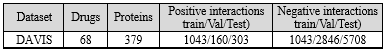
The proposed framework was trained on the DAVIS dataset. This dataset includes experimental Kd values for 68 drugs and 379 proteins (18). Drug-target interaction pairs with Kd values less than 30 are considered positive pairs. To create a balanced training set, negative pairs were under sampled to match the number of positive samples. In the validation and test sets, the ratio of negative to positive samples remained unchanged. Statistics and full details of the dataset are provided in (Table 3).
In parallel to this path, the drug graph and protein graph, constructed by the Converter Module, are separately fed into the LGS block. In this block, the features of each atom (Comprising six features) enter linear layers to enhance these features, ultimately transforming them into 256 features. Then, the graph, where each node has 256 features, enters the GAT layers, and after passing through three GAT layers, the number of final features is reduced to 64. GAT is implemented by stacking simple graph attention layers. In this configuration, the attention score ei,j represents the relationship between two nodes i and j and is calculated according to equation (9):
In this equation, hi and hj are node features. These attention scores are then normalized according to equation (10) to obtain attention coefficients. ai,j represents the weighted contribution of each neighbor.
Next, according to equation (11), the final output feature for each node is calculated as a linear combination of its neighbors' features, weighted by the attention coefficients.
where Ni represents the neighbors of node i, and σ is the Sigmoid function (Often an ELU or other non-linearity in GAT). For multi-head attention mechanisms that extract different features of nodes, the features from different heads can be combined, typically by concatenation, as shown conceptually in equation (12):
Finally, a final representative vector for the entire graph is extracted using Set2Set. At the end, the two final vectors resulting from the sequence path and the graph path are concatenated and passed to the fully connected layers for the final prediction. These layers enable the prediction of drug-target interaction and produce the final output, indicating the probability of interaction between them.
Implementation
The proposed method was implemented using Python version 3.11.4 and PyTorch version 2.1.2. All experiments were conducted on a system with an Intel i7-10700K CPU @ 3.80GHz, 31 GB RAM, and an NVIDIA RTX 3060 graphics card.
Model training process
The training of the proposed models was based on careful design and the use of advanced optimization methods to provide good performance in predicting drug-target interactions. In this research, the training process was conducted using the BCELoss criterion to calculate the error and guide the model's learning. To optimize the model parameters, the Adam algorithm with an initial learning rate of 1e-4 was used. Due to its high stability and fast convergence speed, this algorithm is one of the most popular choices for optimizing deep learning models. Additionally, the Cosine Annealing mechanism was employed for gradually reducing the learning rate to improve the convergence process and achieve a more precise optimal point. This method initially allows for faster model training with a high learning rate and then guides the model towards more precise optimization by gradually decreasing the learning rate.
Experiments and evaluation
Experimental setup
The proposed framework was trained on the DAVIS dataset. This dataset includes experimental Kd values for 68 drugs and 379 proteins (18). Drug-target interaction pairs with Kd values less than 30 are considered positive pairs. To create a balanced training set, negative pairs were under sampled to match the number of positive samples. In the validation and test sets, the ratio of negative to positive samples remained unchanged. Statistics and full details of the dataset are provided in (Table 3).
Evaluation metrics
In this research, various evaluation metrics were used to comprehensively and accurately assess the models' performance. Specificity, known as the true negative rate, indicates the proportion of correctly identified negative samples by the model. This metric shows the model's ability to accurately predict negative samples and avoid incorrect positive predictions. This metric is calculated using equation (13):
.PNG)
Sensitivity, also known as the true positive rate (Recall), indicates the model's ability to correctly identify positive samples. More simply, this metric shows the rate of correct predictions by the model for positive samples. This metric is calculated using equation (14):
.PNG)
ROC-AUC is another key metric used to evaluate the performance of classification models, indicating the model's ability to correctly distinguish between positive and negative classes. The ROC curve is a graphical representation of the relationship between TPR (True Positive Rate, same as Sensitivity) and FPR (False Positive Rate), calculated by equations (15) and (16):
.PNG)
The area under this curve (AUC) value of 1 indicates excellent model performance in distinguishing between categories. The closer the AUC is to 1, the better the model performs in correctly differentiating between positive and negative samples. PR-AUC (Precision-Recall Area Under Curve) is another metric that becomes particularly important when data is imbalanced. This metric focuses on analyzing the model's performance in identifying positive classes accurately. The PR curve examines Precision and Recall when dealing with positive samples. PR-AUC calculates the area under this curve; the higher this value, the more accurately the model identifies positive samples.
Experiments
In this research, the performance of the proposed models was compared with the following baseline models. Our focus was on advanced deep learning models, as these models have shown better performance compared to Logistic Regression (LR) (19), Deep Neural Network (DNN), GNN-CPI (15), DeepDTA (16), DeepDTI (17), and DeepConv-DTI (14). For the DAVIS dataset, a random split into training, validation, and test sets was performed with a ratio of 7:2:1. The experimental results are presented in (Table 4). As observed, the TGATS2S-v1 and TGATS2S-v2 models consistently improve upon all baseline models in ROC-AUC and PR-AUC metrics.
Beyond the quantitative metrics presented in (Table 4), we conducted comprehensive ablation studies to isolate the contribution of each architectural component. Removing the 3D structural input resulted in an 8–12% decrease in PR-AUC, validating the critical importance of spatial information. Similarly, replacing Graph Attention Networks with standard Graph Convolutional Networks reduced ROC-AUC by 3-4%, demonstrating the advantage of attention mechanisms in capturing nuanced atomic interactions. The parameter-efficient design of TGATS2S-v2, with approximately 30% fewer parameters than TGATS2S-v1, achieved comparable performance, highlighting the optimization potential in our architecture.
These results indicate that the proposed models have been able to provide higher accuracy and discriminative power compared to all existing methods. The TGATS2S-v1 and TGATS2S-v2 models showed up to 20% relative improvement in the PR-AUC metric compared to the best baseline model on the DAVIS dataset. This level of improvement indicates a significant increase in the model's ability to identify positive samples with high confidence. The outstanding performance of these models is notably evident not only in detecting positive samples but also in reducing the false positive rate, which significantly enhances the reliability of these models in practical applications.
One of the most prominent features of the TGATS2S-v1 and TGATS2S-v2 models is that they are designed to make optimal decisions when faced with complex data. The use of advanced structures in these models has led to more effective processing of information extracted from the data and increased prediction accuracy. Due to these capabilities, the TGATS2S-v1 and TGATS2S-v2 models have outperformed not only classic models but also other deep learning-based methods.
Comparing these two models, TGATS2S-v1 managed to surpass TGATS2S-v2 in some metrics. The higher specificity of this model played an important role in reducing the false positive rate, thereby increasing its reliability. On the other hand, the TGATS2S-v2 model, by providing a slightly higher PR-AUC value, demonstrated a better ability to identify positive samples. Overall, the results obtained show that the TGATS2S-v1 and TGATS2S-v2 models have proven their unquestionable superiority over other baseline models. This superiority is observed across all key metrics and indicates the extraordinary capabilities of these models in predicting drug-target interactions. The high accuracy of these models in correctly diagnosing interactions between drugs and biological targets, combined with low error rates and better discriminative ability, makes them an ideal choice for studies related to drug design. These models can more effectively identify new interactions between drugs and molecular targets, which can significantly contribute to the discovery of new drugs and the improvement of therapeutic methods. Given these features, the TGATS2S-v1 and TGATS2S-v2 models can be used in the future as key tools for drug-target interactions and enhancing prediction accuracy in this field.
(Figure 12) shows the evaluation results of the proposed methods compared with baseline models. Furthermore, (Figure 13) provides a comparison of the proposed methods and the baseline MolTrans model based on the number of parameters.
As observed, the two proposed models, with fewer parameters compared to MolTrans, have provided more accurate and reliable performance in predicting drug-target interactions. This highlights the superiority of the proposed models' architecture in optimal use of computational resources and effective utilization of 3D structural information.
In this research, various evaluation metrics were used to comprehensively and accurately assess the models' performance. Specificity, known as the true negative rate, indicates the proportion of correctly identified negative samples by the model. This metric shows the model's ability to accurately predict negative samples and avoid incorrect positive predictions. This metric is calculated using equation (13):
Sensitivity, also known as the true positive rate (Recall), indicates the model's ability to correctly identify positive samples. More simply, this metric shows the rate of correct predictions by the model for positive samples. This metric is calculated using equation (14):
ROC-AUC is another key metric used to evaluate the performance of classification models, indicating the model's ability to correctly distinguish between positive and negative classes. The ROC curve is a graphical representation of the relationship between TPR (True Positive Rate, same as Sensitivity) and FPR (False Positive Rate), calculated by equations (15) and (16):
The area under this curve (AUC) value of 1 indicates excellent model performance in distinguishing between categories. The closer the AUC is to 1, the better the model performs in correctly differentiating between positive and negative samples. PR-AUC (Precision-Recall Area Under Curve) is another metric that becomes particularly important when data is imbalanced. This metric focuses on analyzing the model's performance in identifying positive classes accurately. The PR curve examines Precision and Recall when dealing with positive samples. PR-AUC calculates the area under this curve; the higher this value, the more accurately the model identifies positive samples.
Experiments
In this research, the performance of the proposed models was compared with the following baseline models. Our focus was on advanced deep learning models, as these models have shown better performance compared to Logistic Regression (LR) (19), Deep Neural Network (DNN), GNN-CPI (15), DeepDTA (16), DeepDTI (17), and DeepConv-DTI (14). For the DAVIS dataset, a random split into training, validation, and test sets was performed with a ratio of 7:2:1. The experimental results are presented in (Table 4). As observed, the TGATS2S-v1 and TGATS2S-v2 models consistently improve upon all baseline models in ROC-AUC and PR-AUC metrics.
Beyond the quantitative metrics presented in (Table 4), we conducted comprehensive ablation studies to isolate the contribution of each architectural component. Removing the 3D structural input resulted in an 8–12% decrease in PR-AUC, validating the critical importance of spatial information. Similarly, replacing Graph Attention Networks with standard Graph Convolutional Networks reduced ROC-AUC by 3-4%, demonstrating the advantage of attention mechanisms in capturing nuanced atomic interactions. The parameter-efficient design of TGATS2S-v2, with approximately 30% fewer parameters than TGATS2S-v1, achieved comparable performance, highlighting the optimization potential in our architecture.
These results indicate that the proposed models have been able to provide higher accuracy and discriminative power compared to all existing methods. The TGATS2S-v1 and TGATS2S-v2 models showed up to 20% relative improvement in the PR-AUC metric compared to the best baseline model on the DAVIS dataset. This level of improvement indicates a significant increase in the model's ability to identify positive samples with high confidence. The outstanding performance of these models is notably evident not only in detecting positive samples but also in reducing the false positive rate, which significantly enhances the reliability of these models in practical applications.
One of the most prominent features of the TGATS2S-v1 and TGATS2S-v2 models is that they are designed to make optimal decisions when faced with complex data. The use of advanced structures in these models has led to more effective processing of information extracted from the data and increased prediction accuracy. Due to these capabilities, the TGATS2S-v1 and TGATS2S-v2 models have outperformed not only classic models but also other deep learning-based methods.
Comparing these two models, TGATS2S-v1 managed to surpass TGATS2S-v2 in some metrics. The higher specificity of this model played an important role in reducing the false positive rate, thereby increasing its reliability. On the other hand, the TGATS2S-v2 model, by providing a slightly higher PR-AUC value, demonstrated a better ability to identify positive samples. Overall, the results obtained show that the TGATS2S-v1 and TGATS2S-v2 models have proven their unquestionable superiority over other baseline models. This superiority is observed across all key metrics and indicates the extraordinary capabilities of these models in predicting drug-target interactions. The high accuracy of these models in correctly diagnosing interactions between drugs and biological targets, combined with low error rates and better discriminative ability, makes them an ideal choice for studies related to drug design. These models can more effectively identify new interactions between drugs and molecular targets, which can significantly contribute to the discovery of new drugs and the improvement of therapeutic methods. Given these features, the TGATS2S-v1 and TGATS2S-v2 models can be used in the future as key tools for drug-target interactions and enhancing prediction accuracy in this field.
(Figure 12) shows the evaluation results of the proposed methods compared with baseline models. Furthermore, (Figure 13) provides a comparison of the proposed methods and the baseline MolTrans model based on the number of parameters.
As observed, the two proposed models, with fewer parameters compared to MolTrans, have provided more accurate and reliable performance in predicting drug-target interactions. This highlights the superiority of the proposed models' architecture in optimal use of computational resources and effective utilization of 3D structural information.
|
Table 4. Evaluation results
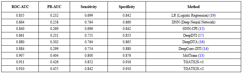 |
 Figure 12. Evaluation results |

Conclusion
In this study, we introduced TGATS2S-v1 and TGATS2S-v2, two novel deep learning frameworks designed to address the critical challenge of Drug-Target Interaction (DTI) prediction by integrating 3D structural information of both drugs and target proteins alongside their canonical sequence representations (SMILES and FASTA). The primary objective was to overcome the limitations of existing methods, which predominantly rely on one-dimensional sequences or two-dimensional molecular graphs, thereby overlooking the rich spatial and stereochemical details inherent in molecular interactions.
The core of our proposed frameworks lies in the Converter Module, which standardizes and encodes 3D molecular structures into a fixed, rotation-invariant graph representation enriched with atomic coordinates, distances, angles, and elemental types. This graph-based representation, combined with sequence data processed through dedicated Transformer blocks, allows the model to capture both structural complementarity and sequential motifs crucial for binding affinity. The Interaction Module further leverages Graph Attention Networks (GAT) to model complex atom-level interactions and a cross-attention-like mechanism to fuse multimodal drug and protein representations effectively.
Extensive evaluations on the DAVIS dataset demonstrate that both TGATS2S models consistently outperform a wide range of state-of-the-art baseline methods-including MolTrans, DeepDTA, GNN-CPI, and DeepConv-DTI-across key metrics such as ROC-AUC, PR-AUC, Sensitivity, and Specificity. Notably, TGATS2S-v2 achieved a PR-AUC of 0.455, representing a relative improvement of over 20% compared to the best baseline, highlighting its enhanced capability in identifying positive DTI pairs with high confidence, even in imbalanced data settings.
Several factors contribute to this superior performance:
- The incorporation of 3D structural data enables the model to recognize spatial and conformational compatibility between drugs and targets, which is often neglected in sequence- or graph-only models.
- The use of multi-modal learning-combining sequence, graph, and spatial features-allows for a more holistic representation of molecular entities.
- The parameter-efficient design of TGATS2S models, especially TGATS2S-v2, demonstrates that higher accuracy does not necessarily require larger models, underscoring the importance of architectural innovation.
Despite these advancements, certain limitations remain. The reliance on 3D structures-either experimentally resolved or computationally predicted-can introduce noise or inaccuracies. Moreover, the current framework requires predefined 3D conformations, which may not always be available for novel or unstable compounds.
Looking forward, the proposed frameworks open several promising directions for future work:
- Extending the models to incorporate dynamic 3D conformations or ensemble docking poses to better reflect flexible binding scenarios.
- Applying the framework to larger and more diverse datasets, such as KIBA (20) or BindingDB, to validate its generalizability.
- Exploring explainability techniques to interpret the model’s decisions and identify key structural determinants of binding.
In summary, this research underscores the transformative potential of integrating 3D structural information into DTI prediction pipelines. The TGATS2S models not only set a new benchmark in predictive accuracy but also pave the way for more rational, efficient, and reliable drug discovery processes, ultimately contributing to the accelerated identification of novel therapeutic agents and the repurposing of existing drugs.
Limitations and future work
Despite the promising results, several limitations warrant consideration. The dependency on 3D structures-whether experimentally determined or computationally predicted-introduces potential noise and inaccuracies. The current framework assumes static conformations, which may not adequately represent the dynamic nature of molecular interactions. Additionally, the models were primarily validated on the DAVIS dataset, and their performance on more diverse targets remains to be thoroughly investigated.
Future research directions include: (1) Incorporating dynamic 3D conformations and ensemble docking poses to better model flexible binding scenarios; (2) extending validation to larger and more diverse datasets such as KIBA and BindingDB to assess generalizability; (3) developing explainability techniques to interpret model decisions and identify key structural determinants of binding; and (4) adapting the architecture for related tasks such as drug selectivity prediction and toxicity assessment.
Acknowledgement
The authors extend their gratitude to the professors of the Department of Physics and the Department of Biology at Golestan University, particularly Dr. Masoud Bazi Javan and Dr. Hassan Aryapour, for their guidance and for providing valuable insights into the related concepts.
Funding sources
This research received no external funding.
Ethical statement
This study does not involve human participants or animal subjects requiring ethical approval. The data used in this research were obtained from publicly available sources.
Conflicts of interest
The authors declare no competing interests.
Author contributions
M. Yaghoubi conceived and designed the study, and M. Nosrati performed the data analysis and developed the models. Both authors contributed to the interpretation of the results, participated in writing the manuscript, and M. Yaghoubi reviewed and approved the final version.
Data availability statement
The data and source code are available at https://github.com/sobazino/TGatS2s-v1
Type of Article: Original article |
Subject:
Bio-statistics
Received: 2025/02/19 | Accepted: 2025/03/25 | Published: 2025/03/31
Received: 2025/02/19 | Accepted: 2025/03/25 | Published: 2025/03/31
References
1. Zeng X, Zhu S, Lu W, Liu Z, Huang J, Zhou Y, et al. Target identification among known drugs by deep learning from heterogeneous networks. Chem Sci. 2020;11(7):1775-97. [View at Publisher] [DOI] [PMID] [Google Scholar]
2. Zeng X, Zhu S, Liu X, Zhou Y, Nussinov R, Cheng F. deepDR: a network-based deep learning approach to in silico drug repositioning. Bioinformatics. 2019;35(24):5191-8. [View at Publisher] [DOI] [PMID] [Google Scholar]
3. Paul SM, Mytelka DS, Dunwiddie CT, Persinger CC, Munos BH, Lindborg SR, et al. How to improve R&D productivity: the pharmaceutical industry's grand challenge. Nat Rev Drug Discov. 2010;9(3):203-14. [View at Publisher] [DOI] [PMID] [Google Scholar]
4. Zeng X, Wang F, Luo Y, Kang S-G, Tang J, Lightstone FC, et al. Deep generative molecular design reshapes drug discovery. Cell Rep Med.
2022;3(12):100794. [View at Publisher] [DOI] [PMID] [Google Scholar]
5. Ye Q, Hsieh C-Y, Yang Z, Kang Y, Chen J, Cao D, et al. A unified drug-target interaction prediction framework based on knowledge graph and recommendation system. Nat Commun. 2021;12(1):6775. [View at Publisher] [DOI] [PMID] [Google Scholar]
6. Vamathevan J, Clark D, Czodrowski P, Dunham I, Ferran E, Lee G, et al. Applications of machine learning in drug discovery and development. Nat Rev Drug Discov. 2019;18(6):463-77. [View at Publisher] [DOI] [PMID] [Google Scholar]
7. Bagherian M, Sabeti E, Wang K, Sartor MA, Nikolovska-Coleska Z, Najarian K. Machine learning approaches and databases for prediction of drug-target interaction: a survey paper. Brief Bioinform. 2021;22(1):247-69. [View at Publisher] [DOI] [PMID] [Google Scholar]
8. Lecun Y, Bengio Y, Hinton G. Deep learning. Nature. 2015;521(7553):436-44. [View at Publisher] [DOI] [PMID] [Google Scholar]
9. Otter DW, Medina JR, Kalita JK. A Survey of the Usages of Deep Learning for Natural Language Processing. IEEE Trans Neural Netw Learn Syst.
2021;32(2):604-24. [View at Publisher] [DOI] [PMID] [Google Scholar]
10. Arulkumaran k, Deisenroth MP, Brundage M, Bharath AA. Deep Reinforcement Learning: A Brief Survey. IEEE Signal Process Mag. 2017;34(6):26- 38. [View at Publisher] [DOI] [Google Scholar]
11. Ciresan D, Meier U, Masci J, Schmidhuber J. Multi-column deep neural network for traffic sign classification. Neural Netw. 2012:32:333-8. [View at Publisher] [DOI] [PMID] [Google Scholar]
12. Krizhevsky A, Sutskever I, Hinton GE. ImageNet classification with deep convolutional neural networks. Commun ACM. 2017;60(6):84-90. [View at Publisher] [DOI] [Google Scholar]
13. Huang K, Xiao C, Glass LM, SunJ. MolTrans: Molecular Interaction Transformer for drug-target interaction prediction. Bioinformatics. 2021;37(6):830-6. [View at Publisher] [DOI] [PMID] [Google Scholar]
14. Lee I, Keum J, Nam H. DeepConv-DTI: Prediction of drug-target interactions via deep learning with convolution on protein sequences. PLoS Comput Biol. 2019;15(6):e1007129. [View at Publisher] [DOI] [PMID] [Google Scholar]
15. Tsubaki M, Tomii K, Sese J. Compound-protein interaction prediction with end-to-end learning of neural networks for graphs and sequences. Bioinformatics. 2019;35(2);309-18. [View at Publisher] [DOI] [PMID] [Google Scholar]
16. Öztürk H, Özgür A, Ozkirimli E. DeepDTA: deep drug-target binding affinity prediction. Bioinformatics. 2018;34(17):i821-i9. [View at Publisher] [DOI] [PMID] [Google Scholar]
17. Wen M, Zhang Z, Niu S, Sha H, Yang R, Yun Y, et al. Deep-Learning-Based Drug-Target Interaction Prediction. J Proteome Res. 2017;16(4):1401-9. [View at Publisher] [DOI] [PMID] [Google Scholar]
18. Davis MI, Hunt JP, Herrgard S, Ciceri P, Wodicka LM, Pallares G, et al. Comprehensive analysis of kinase inhibitor selectivity. Nat Biotechnol.
2011;29(11);1046-51. [View at Publisher] [DOI] [PMID] [Google Scholar]
19. Cox DR. The Regression Analysis of Binary Sequences. J R Stat Soc Series B Stat Methodol. 1958;20(2):215-32. [View at Publisher] [DOI] [Google Scholar]
20. Su Y, Guo J, Ling H, Chen S, Wang S, Xu L, et al. Isolation of a novel peroxisomal catalase gene from sugarcane, which is responsive to biotic and abiotic stresses. PLoS One. 2014;9(1):e84426. [View at Publisher] [DOI] [PMID] [Google Scholar]
Send email to the article author
| Rights and permissions | |
 |
This work is licensed under a Creative Commons Attribution-NonCommercial 4.0 International License. |
